Feedforward and Backward Propagation in Gated Recurrent Unit (GRU)
Published:
In this post, I’ll discuss how to implement a simple Recurrent Neural Network (RNN), specifically the Gated Recurrent Unit (GRU). I’ll present the feed forward proppagation of a GRU Cell at a single time stamp and then derive the formulas for determining parameter gradients using the concept of Backpropagation through time (BPTT).
Forward Propagation
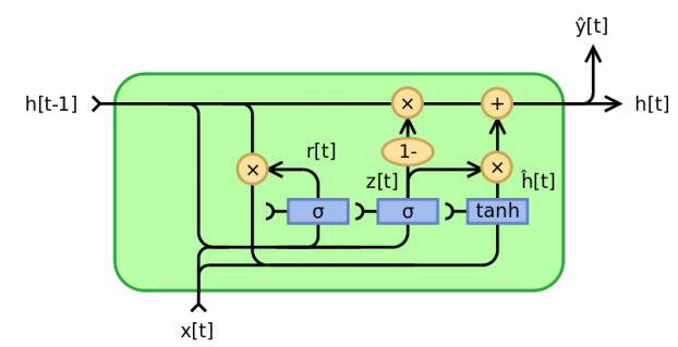
The feedforward propagation equations for a GRU cell are expressed as:
\[z_t = \sigma(W_{zh}\ast h_{t-1} + W_{zx}\ast x_t)\] \[r_t = \sigma(W_{rh}\ast h_{t-1} + W_{rx}\ast x_t)\] \[\tilde{h}_t = f(W_h\ast (r_t \circ h_{t-1}) + W_x\ast x_t)\] \[h_t = z_t\circ h_{t-1} + (1-z_t)\circ \tilde{h}_t,\]where $x_t$ is the input vector at time $t$, $h_t$ is the output vector, $\ast$ denotes matrix product, $\circ$ denotes element-wise product, $\sigma$ and $f$ are the sigmoid and Tanh activation functions, respectively.
Backward Propagation
Lets rewrite these set of equation in terms of unary and binary operations following the same order.
\[g_1 = W_{zh} \ast h_{t-1}\] \[g_2 = W_{zx} \ast x_{t}\] \[g_3 = g_1 + g_2\] \[z_t = \sigma(g_3)\] \[g_4 = W_{rh} \ast h_{t-1}\] \[g_5 = W_{rx} \ast x_{t}\] \[g_6 = g_4 + g_5\] \[r_t = \sigma(g_6)\] \[g_7 = r_t \circ h_{t-1}\] \[g_8 = W_{h} \ast g_7\] \[g_9 = W_{x} \ast x_{t}\] \[g_{10} = g_8 + g_9\] \[\tilde{h}_t = f(g_{10})\] \[g_{11} = z_t\circ h_{t-1}\] \[g_{12} = (1-z_t)\circ \tilde{h}_t\] \[h_t = g_{11} + g_{12}\]Now, we’‘ll work our way backward to compute the parameter gradients, i.e. the derivatives of loss $L$ with respect to parameters. Let assume that gradient of loss with repect to output is known and denoted as $\Delta_{h_t}L$.
- Eq. (20) gives
- Eq. (19) gives
- Eq. (18) gives
Second time we’re computing a derivative for $z_t$, so we increment the derivative $(+=)$.
- Eq. (17) gives
- Eq. (16) gives
- Eq. (15) gives
- Eq. (14) gives
- Eq. (13) gives
- Eq. (12) gives
- Eq. (11) gives
- Eq. (10) gives
- Eq. (9) gives
- Eq. (8) gives
- Eq. (7) gives
- Eq. (6) gives
- Eq. (5) gives
This completes all the required formulas for computing derivative with respect to all the parameters of network.